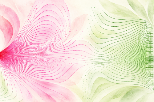
1. Introduction — An unexpected poetic geometry
Alcoholometric tables are among the everyday tools used by professionals in the spirits industry. In particular, they allow an alcoholic strength by volume (ABV) reading taken at a temperature other than 20 °C to be corrected to the reference temperature of 20 °C.
However, when we examine not the numerical values themselves, but the differences between successive values, surprising patterns emerge: networks of curved lines resembling flower petals or clover leaves.
This article offers a different perspective on alcoholometric tables. After reviewing the principles used to correct ABV readings obtained with an alcohol hydrometer, we will explore how graphical analysis of the data can reveal these unexpected patterns, while also helping to detect certain transcription errors in published tables.
Finally, we will examine how these patterns originate from the complex physical properties of a mixture as familiar as water and ethanol.
2. Why correct an alcohol hydrometer reading ?
The alcoholic strength by volume (ABV) read on an alcohol hydrometer depends on the temperature of the liquid. This phenomenon is mainly related to the expansion or contraction of the water–ethanol mixture as its temperature changes.
The magnitude of the correction depends on both the measurement temperature and the alcoholic strength of the liquid. Since the reference temperature is set at 20 °C, any reading taken at a different temperature must be corrected to obtain the ABV at 20 °C.
For this purpose, professionals use, in particular, table VIIIb from Mr Oudin’s Guide pratique d’alcoométrie [1], or the table published by the European Commission in volume 1: Practical alcoholic-stength tables [2].
3. Origin of Table VIIIb and its use
This table is based on the provisions of International Recommendation R 22, published by the International Organization of Legal Metrology (OIML) [3].
This recommendation includes an equation for calculating the density of water–ethanol mixtures as a function of their composition and temperature, as well as the calculation methods used to establish the various alcoholometric tables.
The resulting Table VIIIb makes it possible to correct the ABV reading obtained with a soda-lime glass volumetric alcohol hydrometer, taking into account both the physical properties of the water–ethanol mixture and the thermal expansion of the instrument.
4. An observation arising from the computerization of alcoholometric tables
In 2015, while working on the traceability and computerization of alcoholometric tables, I revisited the OIML R 22 model and its specifications with the assistance of software engineers. This made it possible to calculate values with greater precision than those in printed tables, compare different editions, and identify transcription errors. This work was published in the OIML Bulletin [4].
A black-and-white graphical representation published at that time already revealed unexpected patterns. I recently revisited this observation by assigning colours to the differences between two successive corrected ABV values, at a constant temperature, for an increment of 0.1% vol. in the ABV reading.
Figure 1 presents the data graphically. The coloured points align to form networks of parallel curves, creating patterns reminiscent of botanical shapes.
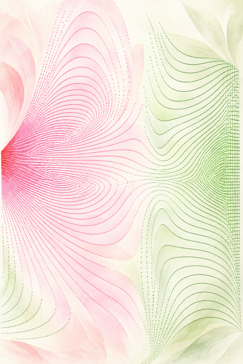
Figure 2 offers an artistic interpretation of these patterns, intended to highlight this resemblance. It is therefore an illustration rather than an additional representation of measured or calculated data.
Figure 1 — Increments from Table VIIIb of the Guide pratique d’alcoométrie
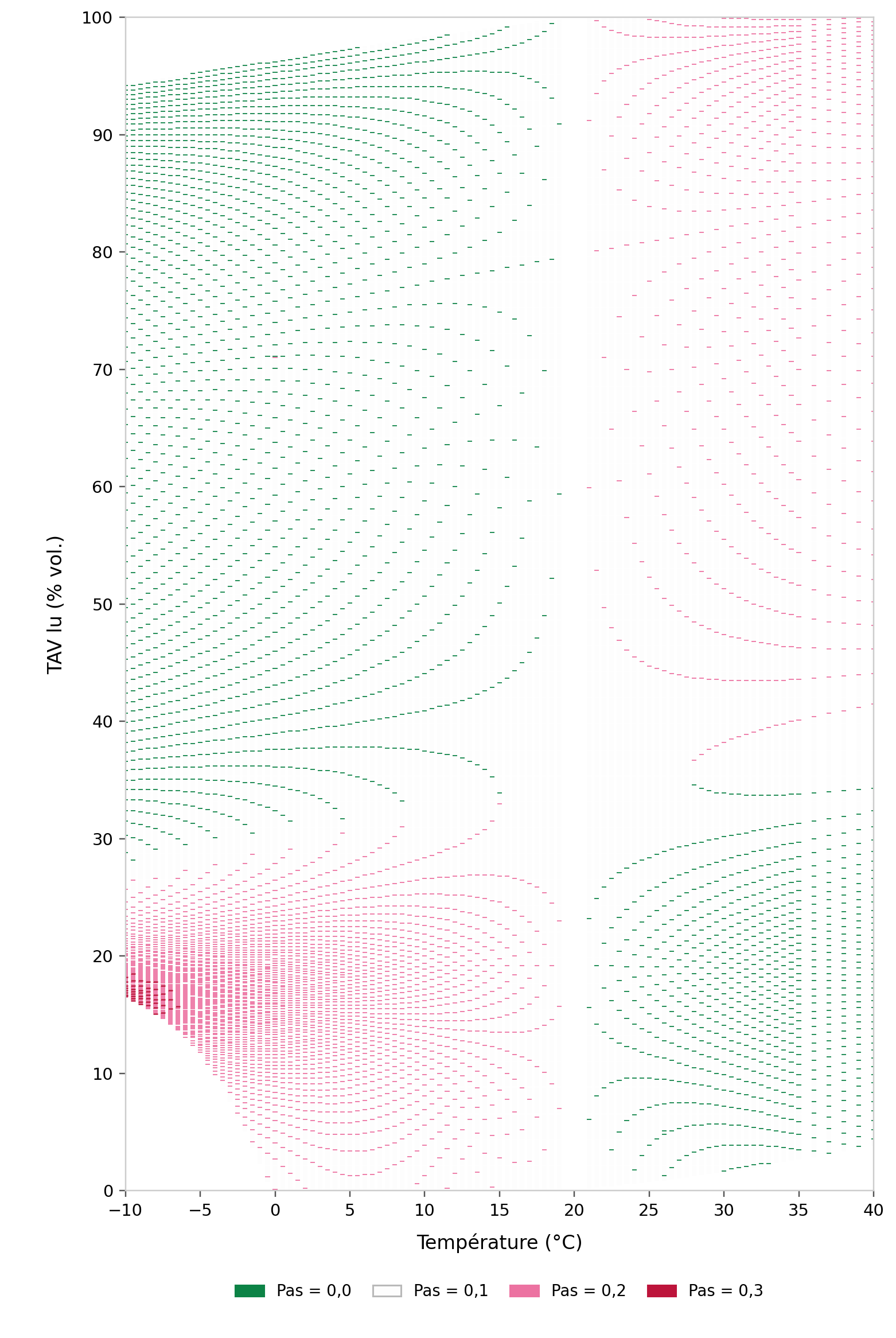
Figure 2 — Artistic interpretation inspired by Figure 1
5. A suspicious discrepancy revealed by these graphs
The graphical representation of the increments (Figure 1) also makes it possible to identify potential anomalies when comparing printed tables with calculated values.
For example, in the 6th edition of the Guide pratique d’alcoométrie, at a temperature of 0 °C, Figure 1 reveals a suspicious discrepancy of 0.2% vol.: the corrected ABV increases from 77.1 to 77.3% vol. when the ABV reading on the alcohol hydrometer increases from 70.9 to 71.0% vol.
However, the conversions to 20 °C, calculated using the OIML reference equations, give 77.11 and 77.20% vol., respectively, corresponding to an actual increment of 0.09% vol.
Figure 3 below shows an enlargement of the corresponding area of Figure 1. A red line, representing an increment of 0.2% vol., stands out from the other lines in this area, which are all green and correspond to increments of 0.1% vol.
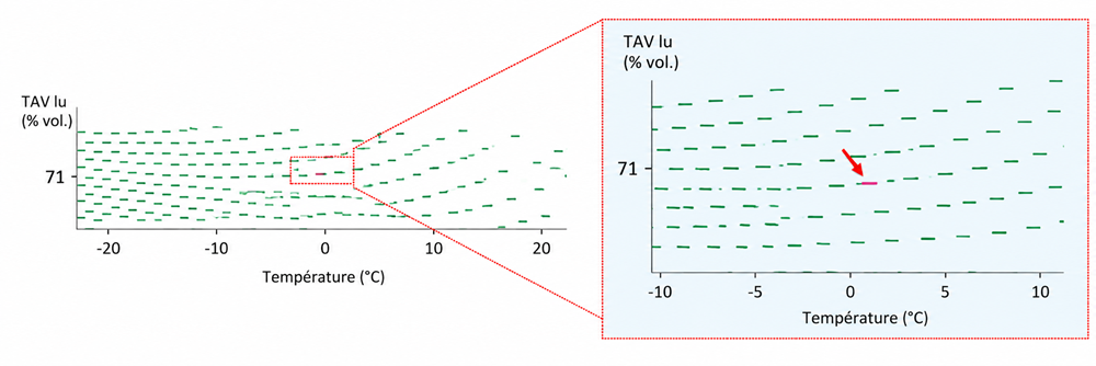
After rounding to one decimal place, the expected values are therefore 77.1 and 77.2% vol., corresponding to an increment of 0.1% vol., rather than 0.2% vol.
This example thus highlights a probable transcription error in the edition concerned, rather than a simple effect of the rounding rules.
For accurate and reliable alcoholometric conversions, use the online tool: Labox alcoholemetry
6. Where do the observed patterns come from?
6.1. A liquid with non-linear properties
As professionals in the spirits industry know well, mixing water and ethanol is not simply a matter of adding their volumes together. The molecules interact, particularly through hydrogen bonding: the mixture can undergo volume contraction, and its thermal expansion depends on its composition. Density therefore does not vary in a simply proportional manner with temperature or ABV. These properties are discussed in my article “Blending eaux-de-vie: a rather strange contraction phenomenon” (January 16, 2024) [5].
6.2. Rounding reveals patterns of alignment
Printed tables present results rounded to the nearest 0.1% vol. When two already rounded values are subtracted, the resulting difference may be 0, 0.1, 0.2, and sometimes 0.3% vol. These categories depend both on the actual difference and on the position of the two values relative to the rounding thresholds.
These thresholds are not crossed randomly: their crossings follow the regular but non-linear variations of the alcoholometric function. Patterns of aligned points emerge and, once coloured, resemble flower petals.
The precise shape of these patterns also depends on the step size used to construct the table, both for temperature and for the ABV reading. Changing this step size can shift the alignment of the points and alter the appearance of the botanical patterns, without any corresponding change in the physical properties of the water–ethanol mixture.
6.3. What if we remove the rounding?
The tables recalculated by LABOX Applications provide ABV correction values to several decimal places.
We therefore calculated the differences between two successive corrected ABV values directly from these unrounded values, for an increase of 0.1% vol. in the ABV reading, at a constant temperature.
Unlike the increments in printed tables, which fall into four categories (0, 0.1, 0.2 and 0.3% vol.), these unrounded increments vary continuously with temperature and the ABV reading.
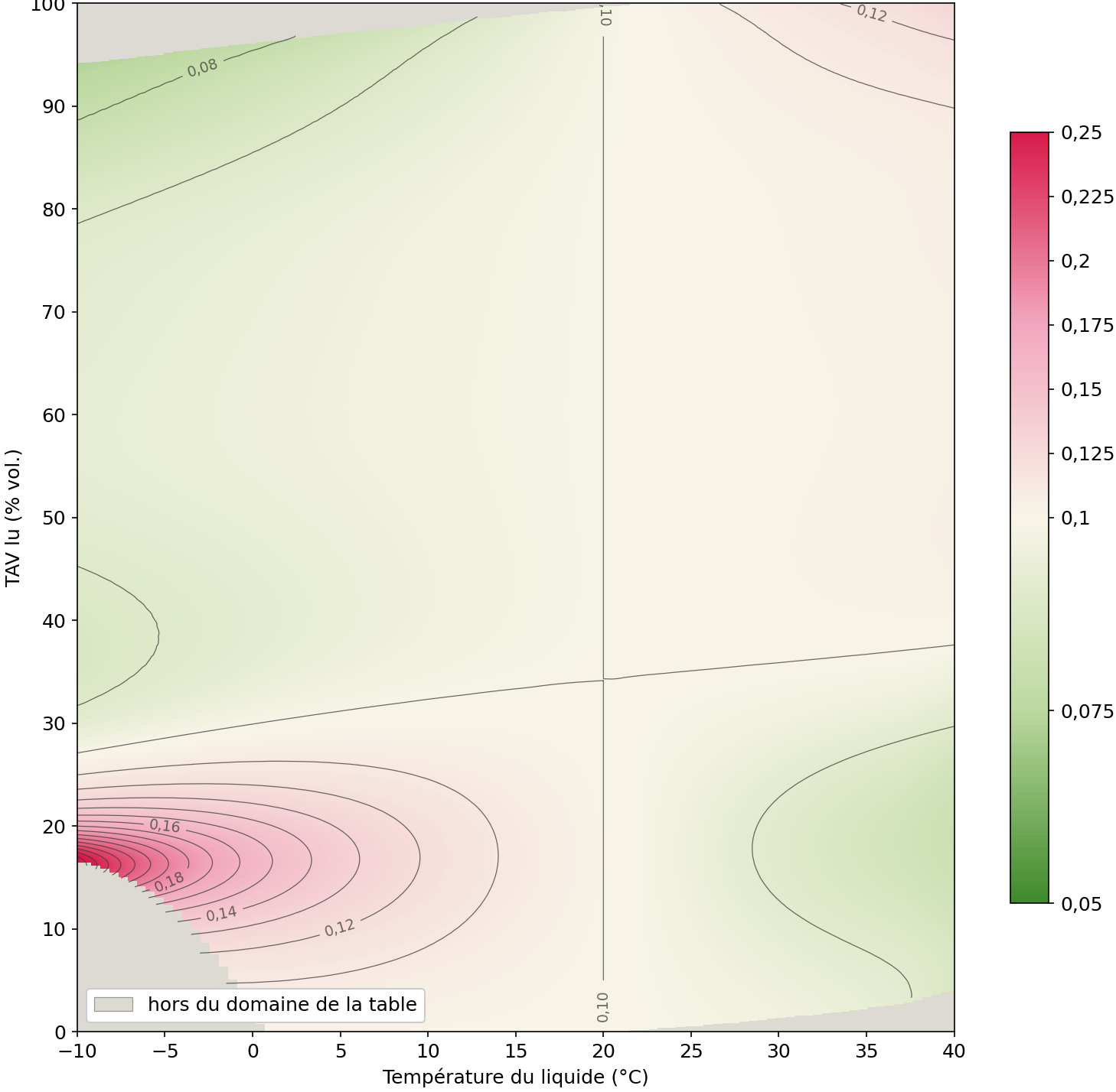
Figure 4 illustrates these variations as a colour map, with contour lines connecting points having the same increment.
The green areas correspond to increments below 0.1% vol., the pink areas to increments above this value, while the cream-coloured areas represent values close to 0.1% vol.
This continuous representation thus provides a better understanding of the variations in the alcoholometric function that contribute to the emergence of the botanical patterns revealed by rounding in Figure 1.
Figure 4 – ABV correction increments based on OIML R 22 data, calculated at intervals of 0.1% vol.
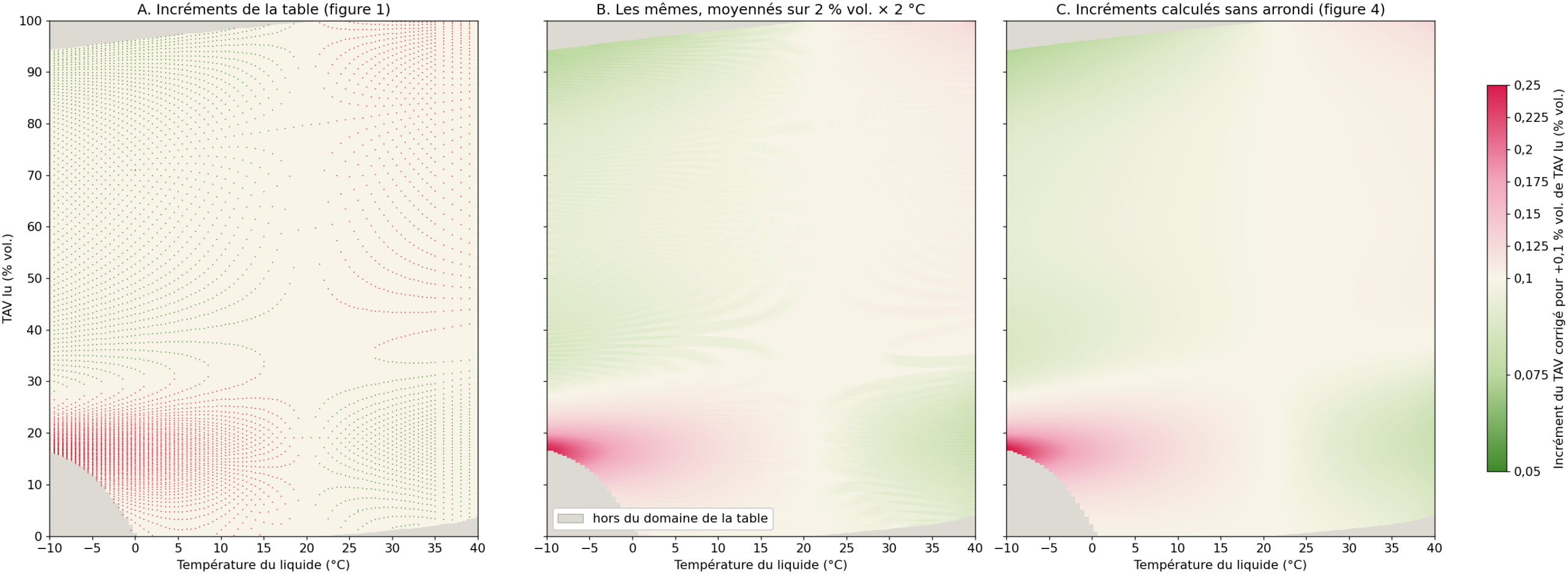
A second data processing method, illustrated in Figure 5, provides a better understanding of the relationship between the previous representations. It compares the increments derived from the rounded values in Table VIIIb (A), corresponding to Figure 1, the same increments after graphical smoothing (B), and the increments calculated without rounding using the OIML model (C), corresponding to Figure 4.
Smoothing reduces the variations caused by rounding and reveals regions of similar behaviour to those obtained from unrounded values.
This comparison illustrates how the botanical patterns emerge from the combination of the continuous variations of the alcoholometric model, the rounding rules and the calculation grid, although it does not, in itself, provide a definitive demonstration of their exact origin.
Figure 5
7. What these images reveal — and their limitations
The figures highlight the interaction between two phenomena: the physical properties of the water–ethanol mixture determine the continuous variation of alcoholometric corrections, while rounding these values to one decimal place produces discontinuous geometric patterns.
Beyond their aesthetic appeal and their usefulness in detecting potential anomalies in the tables, these graphical representations could also serve as a starting point for further scientific investigations.
Figure 4, based on unrounded values, shows how the increment in corrected ABV varies for an increase of 0.1% vol. in the ABV reading, at a constant temperature. It reveals regions where this increment changes relatively little with temperature and ethanol concentration, and others where its variations are more pronounced, as indicated by the closer spacing or changes in orientation of the contour lines.
These differences show how the corrected ABV changes and indirectly reflect the non-linear thermophysical behaviour of water–ethanol mixtures.
Note: Although these graphical representations do not, on their own, allow the identification of specific molecular structures or defined associations of water and ethanol molecules, they could nevertheless guide further studies into the physical properties of these mixtures.
However, as explained in my blog article “Blending eaux-de-vie: a rather strange contraction phenomenon”, for such studies, it would be preferable to express the composition of the mixture in terms of mass fraction, or even mole fraction, rather than alcoholic strength by volume. The latter, conventionally defined at a reference temperature, does not directly reflect the molecular proportions of the mixture, particularly because of the phenomenon of volume contraction.
8. Conclusion — The unexpected beauty of Table VIIIb
Designed to correct alcoholic strength by volume readings taken with an alcohol hydrometer to the reference temperature of 20 °C, the correction table also reveals an unexpected geometry.
Beyond their aesthetic appeal, these graphical representations also serve as a verification tool: they make it possible to identify irregularities that may reveal transcription errors in alcoholometric tables.
Graphical analysis of unrounded data also provides a clearer visualization of variations in the alcoholometric model and could suggest new avenues for studying the thermophysical properties of water–ethanol mixtures.
These “botanical patterns” do not, however, exist within the liquid itself: they arise from the interplay between the complex physical properties of water–ethanol mixtures, their representation by the OIML equations, and the numerical rules used to construct the tables.
They invite us to look at the numbers we use every day from a different perspective.
Evelyne CHANSON –Consultant in quality control of Wines and Spirits of EC Consulting
Did you enjoy this article? If it raises any need for additional information or corrections, feel free to let me know,
by mail: evelyne.chanson@gmail.com or in the comments section at the bottom of this article.
References cited in the article
[1] Guide Pratique d’alcoométrie – P. OUDIN
[2] Practical alcoholic-stength tables – Volume 1 – European Commission
[3] OIML R 22:1975 — INTERNATIONAL ALCOHOLOMETRIC TABLES https://www.oimlsmart.org/publications/pub/r22-1975-e/
[4] E. Chanson, « Traceability and computerization of alcoholometric tables », OIML Bulletin, vol. LVI, n° 3, juillet 2015, p. 5 et suiv. https://www.oiml.org/en/publications/bulletin/pdf/oiml_bulletin_july_2015.pdf
0 Comments